2024 AP Calculus BC Free-Response Questions

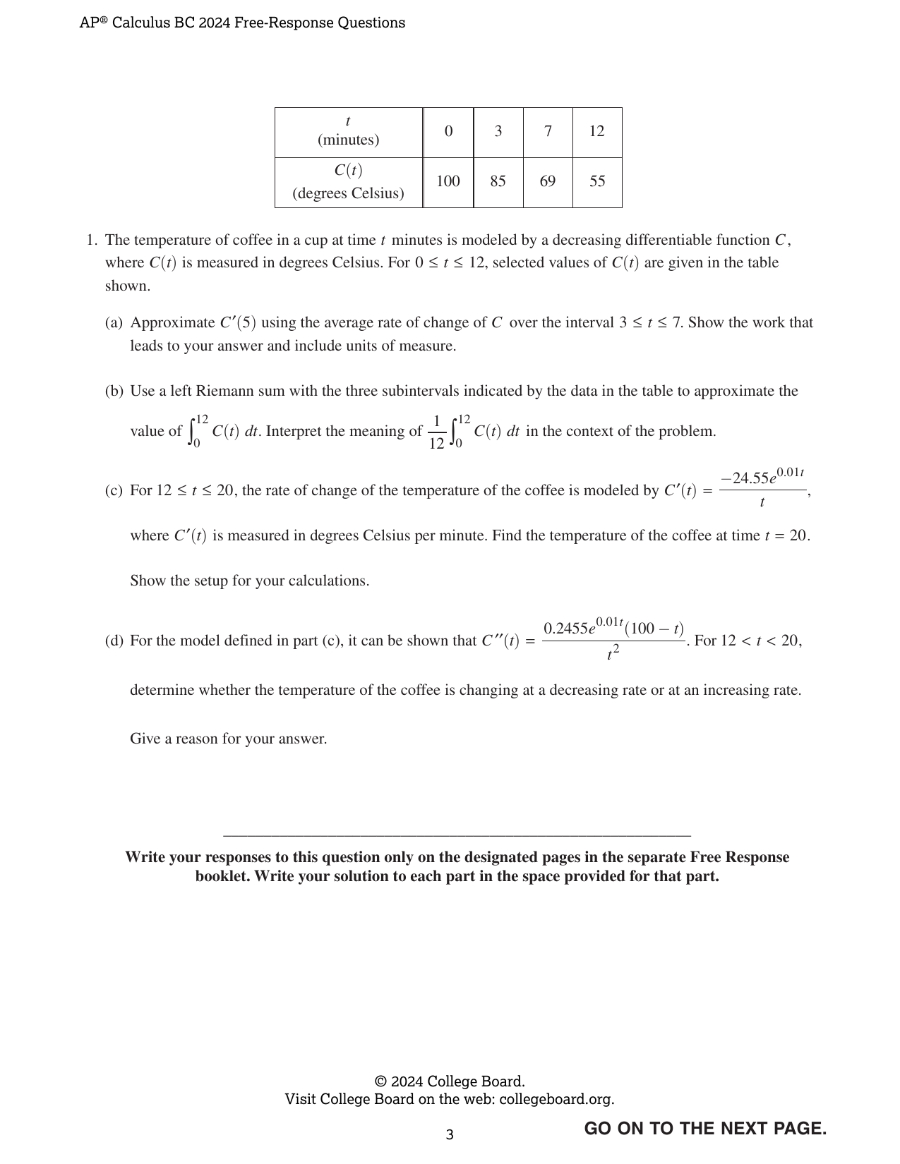
The temperature of coffee in a cup at time t minutes is modeled by a decreasing differentiable function C, where C(t) is measured in degrees Celsius. For 0 ≤ t ≤ 12, selected values of C(t) are given in the table shown. t (minutes) | 0 | 3 | 7 | 12 C(t) (degrees Celsius) | 100 | 85 | 69 | 55 (a) Approximate C′(5) using the average rate of change of C over the interval 3 ≤ t ≤ 7. Show the work that leads to your answer and include units of measure. (b) Use a left Riemann sum with the three subintervals indicated by the data in the table to approximate the value of ∫₀¹² C(t) dt. Interpret the meaning of (1/12)∫₀¹² C(t) dt in the context of the problem. (c) For 12 ≤ t ≤ 20, the rate of change of the temperature of the coffee is modeled by C′(t) = −(24.55e⁰·⁰¹ᵗ)/t, where C′(t) is measured in degrees Celsius per minute. Find the temperature of the coffee at time t = 20. Show the setup for your calculation. (d) For the model defined in part (c), it can be shown that C″(t) = [0.2455e⁰·⁰¹ᵗ(100 − t)]/t². For 12 < t < 20, determine whether the temperature of the coffee is changing at a decreasing rate or at an increasing rate. Give a reason for your answer. Write your responses to this question only on the designated pages in the separate Free Response booklet. Write your solution to each part in the space provided for that part.

2. A particle moving along a curve in the xy-plane has position (x(t), y(t)) at time t seconds, where x(t) and y(t) are measured in centimeters. It is known that x′(t) = 8t − t² and y′(t) = −t + √(t^1.2 + 20). At time t = 2 seconds, the particle is at the point (3, 6). (a) Find the speed of the particle at time t = 2 seconds. Show the setup for your calculations. (b) Find the total distance traveled by the particle over the time interval 0 ≤ t ≤ 2. Show the setup for your calculations. (c) Find the y-coordinate of the position of the particle at the time t = 0. Show the setup for your calculations. (d) For 2 ≤ t ≤ 8, the particle remains in the first quadrant. Find all times t in the interval 2 ≤ t ≤ 8 when the particle is moving toward the x-axis. Give a reason for your answer. Write your responses to this question only on the designated pages in the separate Free Response booklet. Write your solution to each part in the space provided for that part.

3. The depth of seawater at a location can be modeled by the function H that satisfies the differential equation \(\frac{dH}{dt}=\frac{1}{2}(H-1)\cos\left(\frac{t}{2}\right)\), where \(H(t)\) is measured in feet and \(t\) is measured in hours after noon (\(t=0\)). It is known that \(H(0)=4\). (a) A portion of the slope field for the differential equation is provided. Sketch the solution curve, \(y=H(t)\), through the point \((0,4)\). [Provided slope field with axes \(t\) and \(y\), and the point \((0,4)\).] (b) For \(0<t<5\), it can be shown that \(H(t)>1\). Find the value of \(t\), for \(0<t<5\), at which \(H\) has a critical point. Determine whether the critical point corresponds to a relative minimum, a relative maximum, or neither a relative minimum nor a relative maximum of the depth of seawater at the location. Justify your answer. (c) Use separation of variables to find \(y=H(t)\), the particular solution to the differential equation \(\frac{dH}{dt}=\frac{1}{2}(H-1)\cos\left(\frac{t}{2}\right)\) with initial condition \(H(0)=4\).

4. The graph of the differentiable function f, shown for −6 ≤ x ≤ 7, has a horizontal tangent at x = −2 and is linear for 0 ≤ x ≤ 7. Let R be the region in the second quadrant bounded by the graph of f, the vertical line x = −6, and the x- and y-axes. Region R has area 12. [Graph of f: the curve passes through (−6, 0.5), has a horizontal tangent at x = −2, and meets the y-axis at y = 2. For 0 ≤ x ≤ 7, the graph is a line passing through (0, 2), (4, 0), and (6, −1). The shaded region R is bounded by the graph of f, x = −6, the x-axis, and the y-axis.] (a) The function g is defined by g(x) = ∫₀ˣ f(t) dt. Find the values of g(−6), g(4), and g(6). (b) For the function g defined in part (a), find all values of x in the interval 0 ≤ x ≤ 6 at which the graph of g has a critical point. Give a reason for your answer. (c) The function h is defined by h(x) = ∫₋₆ˣ f′(t) dt. Find the values of h(6), h′(6), and h″(6). Show the work that leads to your answers.

5. The function f is twice differentiable for all x with f(0)=0. Values of f′, the derivative of f, are given in the table for selected values of x. Table: x | 0 | π | 2π f′(x) | 5 | 6 | 0 (a) For x ≥ 0, the function h is defined by h(x)=∫₀ˣ√(1+(f′(t))²) dt. Find the value of h′(π). Show the work that leads to your answer. (b) What information does ∫₀^π√(1+(f′(x))²) dx provide about the graph of f? (c) Use Euler’s method, starting at x = 0 with two steps of equal size, to approximate f(2π). Show the computations that lead to your answer. (d) Find ∫(t + 5)cos(t/4) dt. Show the work that leads to your answer.

6. The Maclaurin series for a function f is given by \(\sum_{n=1}^{\infty} \frac{(n+1)x^n}{n^2 6^n}\) and converges to \(f(x)\) for all \(x\) in the interval of convergence. It can be shown that the Maclaurin series for \(f\) has a radius of convergence of 6. (a) Determine whether the Maclaurin series for \(f\) converges or diverges at \(x=6\). Give a reason for your answer. (b) It can be shown that \(f(-3)=\sum_{n=1}^{\infty}\frac{(n+1)(-3)^n}{n^2 6^n}=\sum_{n=1}^{\infty}\frac{n+1}{n^2}\left(-\frac{1}{2}\right)^n\) and that the first three terms of this series sum to \(S_3=-\frac{125}{144}\). Show that \(|f(-3)-S_3|<\frac{1}{50}\). (c) Find the general term of the Maclaurin series for \(f'\), the derivative of \(f\). Find the radius of convergence of the Maclaurin series for \(f'\). (d) Let \(g(x)=\sum_{n=1}^{\infty}\frac{(n+1)x^{2n}}{n^2 3^n}\). Use the ratio test to determine the radius of convergence of the Maclaurin series for \(g\).