2023 AP Macroeconomics Free-Response Questions
Advanced PlacementAP MacroeconomicsEconomicsFree Response
3 questions20 pts
3 gradable20 rubric criteria0 dependencies
q1Question 1
q1
Question 1
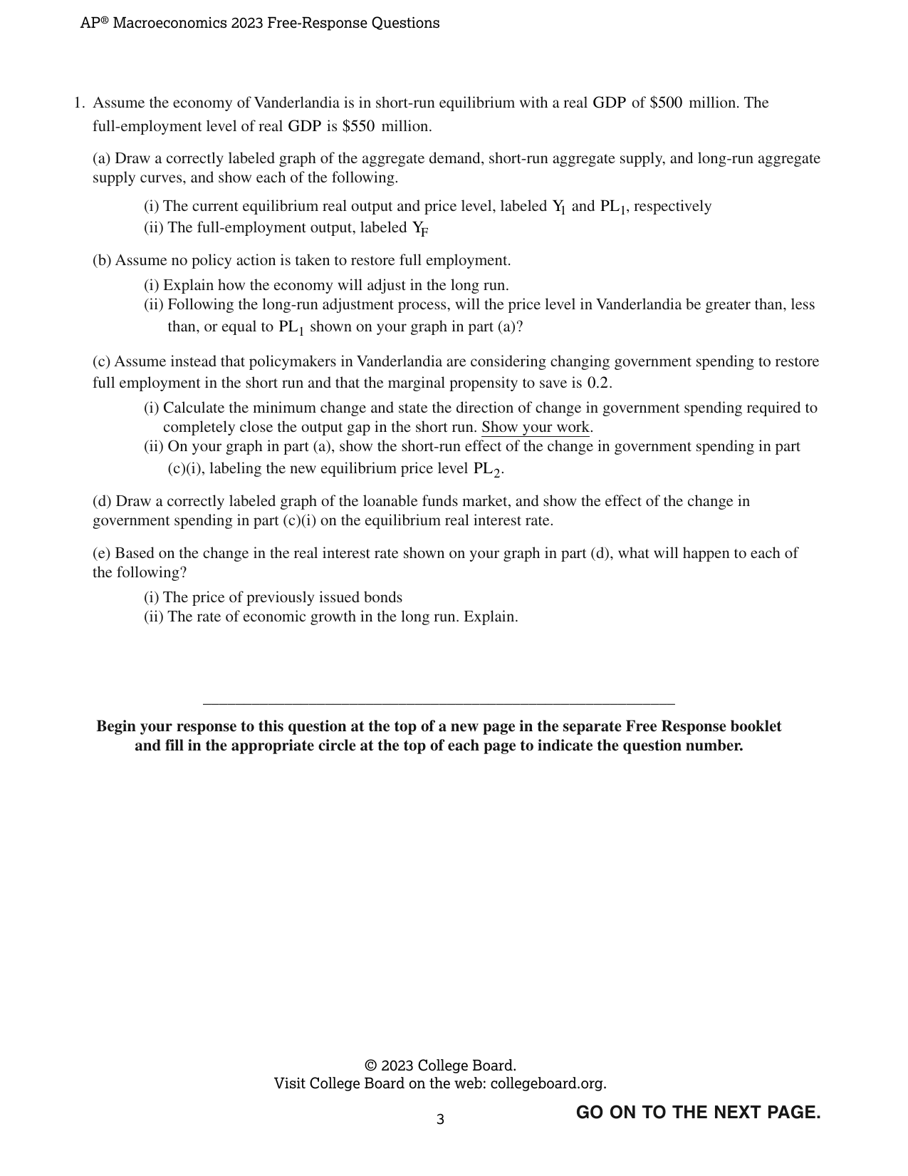
1. Assume the economy of Vanderlandia is in short-run equilibrium with a real GDP of $500 million. The full-employment level of real GDP is $550 million. (a) Draw a correctly labeled graph of the aggregate demand, short-run aggregate supply, and long-run aggregate supply curves, and show each of the following. (i) The current equilibrium real output and price level, labeled Y₁ and PL₁, respectively (ii) The full-employment output, labeled Y_F (b) Assume no policy action is taken to restore full employment. (i) Explain how the economy will adjust in the long run. (ii) Following the long-run adjustment process, will the price level in Vanderlandia be greater than, less than, or equal to PL₁ shown on your graph in part (a)? (c) Assume instead that policymakers in Vanderlandia are considering changing government spending to restore full employment in the short run and that the marginal propensity to save is 0.2. (i) Calculate the minimum change and state the direction of change in government spending required to completely close the output gap in the short run. Show your work. (ii) On your graph in part (a), show the short-run effect of the change in government spending in part (c)(i), labeling the new equilibrium price level PL₂. (d) Draw a correctly labeled graph of the loanable funds market, and show the effect of the change in government spending in part (c)(i) on the equilibrium real interest rate. (e) Based on the change in the real interest rate shown on your graph in part (d), what will happen to each of the following? (i) The price of previously issued bonds (ii) The rate of economic growth in the long run. Explain. Begin your response to this question at the top of a new page in the separate Free Response booklet and fill in the appropriate circle at the top of each page to indicate the question number.
Rubric Criteria (10)
C1Draw a correctly labeled aggregate demand–aggregate supply graph that shows PL1 and Y1 at the intersection of aggregate demand and short-run aggregate supply.
1.0000pts
C2Show a vertical long-run aggregate supply curve to the right of Y1 on the aggregate demand–aggregate supply graph and label the full-employment output as YF.
1.0000pts
C3Explain that input prices (e.g., nominal wages) and/or inflationary expectations will decrease, causing SRAS to increase until it reaches full employment.
1.0000pts
C4State that the price level will be less than PL1.
1.0000pts
C5Calculate the minimum change in government spending as an increase of $10 million and show your work.
1.0000pts
C6On the aggregate demand–aggregate supply graph from part (a), show the short-run effect of the change in government spending as a rightward shift of the aggregate demand curve where the new short-run equilibrium intersects the long-run aggregate supply curve at a higher equilibrium price level, labeled PL2.
1.0000pts
C7Draw a correctly labeled graph of the loanable funds market.
1.0000pts
C8Show an increase in the demand for loanable funds or a decrease in the supply of loanable funds on the loanable funds market graph, resulting in an increase in the equilibrium real interest rate.
1.0000pts
C9State that the price of previously issued bonds will decrease.
1.0000pts
C10State that the rate of economic growth in the long run will decrease and explain that an increase in the real interest rate means the cost of borrowing has increased, which will decrease investment spending on physical capital, human capital, and/or research and development.
1.0000pts
Dependencies (0)
Page Mapping (1)
Visual Preview
15 boxes
Draw, drag, resize. Advanced coordinates are available if needed.
1
2
3
4
5
6
7
8
9
10
11
12
13
14
15
Select a box to edit its role and metadata.
Attribution
This material is the intellectual property of College Board, is not owned by GradeThis, and is shown here for ease of use and demonstration purposes.